Sinusoidal steady state analysis: Phasors & Derivations | Network Theory (Electric Circuits) - Electrical Engineering (EE) PDF Download

Sinusoidal steady-state analysis is a key method in electrical engineering for assessing circuits driven by sinusoidal AC sources at a consistent frequency. It simplifies the analysis of time-varying signals by representing voltages and currents as phasors, which are complex numbers that encode both magnitude and phase, and allows engineers to determine critical circuit properties like impedance and power once transients have subsided, such as when a capacitor reaches a fully charged state with zero current.
- Phasor Representation: This technique transforms complex, time-dependent sinusoidal voltages and currents into phasors, making it easier to analyze circuit behavior without dealing with detailed time-domain mathematics.
- Steady-State Properties: It enables the calculation of essential characteristics like impedance, power, and voltage-current relationships in steady-state conditions, providing insight into circuit performance under continuous sinusoidal operation.
What Is Sinusoidal Steady State Analysis?
Sinusoidal steady-state analysis is a method used to examine electrical circuits after the initial transient phase has passed, leaving the circuit in a stable, oscillating state where all voltages and currents are sinusoidal with a uniform frequency. In this equilibrium, the amplitudes and phases of these signals remain constant over time, enabling their representation as phasors—complex numbers that simplify the analysis. This approach allows engineers to apply familiar tools like Kirchhoff’s laws and nodal analysis to AC circuits in a manner similar to DC circuits, making it particularly useful for studying systems powered by AC sources or signal generators.
- Phasor Simplification: By representing steady-state sinusoidal voltages and currents as phasors, this technique reduces complex time-varying signals into manageable complex numbers, streamlining the analytical process.
- Circuit Law Application: It permits the use of standard circuit analysis methods, such as Kirchhoff’s laws and node equations, on AC circuits, treating them similarly to DC circuits for efficient evaluation.
Sinusoidal Source
A sinusoidal source is critical for sinusoidal steady-state analysis, supplying the circuit with a steady sinusoidal voltage or current, such as a sine wave from a function generator or the sinusoidally varying output of a power system. This source is assumed to produce a pure sinusoid at a single frequency, devoid of harmonics, which drives the circuit into a stable oscillating state where all voltages and currents oscillate at the same frequency. Once this steady state is achieved, the circuit’s response can be efficiently analyzed using phasors, simplifying the evaluation of its behavior under these conditions.
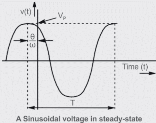
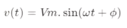
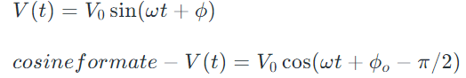
This equation describes the sinusoidal voltage:
 where v(t) is the instantaneous voltage at time t.
- Vm is the amplitude or peak voltage
- w is the angular frequency t is time.
- ϕ is the phase angle
Since,
f=1/T
𝜔=2𝜋𝑓=2𝜋/𝑇
𝑣(𝑡)=𝑉𝑚.sin(𝜔𝑡+𝜙)
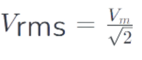
The coefficient of 𝑉𝑚 in the above equation represents the maximum amplitude of the sinusoidal voltage, as cosine oscillates between the bounds of +𝑉𝑚 and −𝑉𝑚, defining the amplitude range.
The illustrated figure clarifies these characteristics. Meanwhile, the angle Φ denotes the phase angle of the sinusoidal voltage, calculated as the square root of the mean value of the square function.
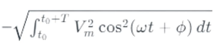
The above equation minimizes

Now,
Steady state sinusoidal analysis using phasors
Phasors allow representing sinusoidal voltages and currents as complex numbers where the magnitude is the peak value and the angle is the phase. This transforms a time-varying AC circuit into an equivalent circuit of phase angles and impedances that can be analyzed using ordinary algebraic and graphical methods.
First, all voltages and currents are expressed as the sum of a sinusoid and its complex exponential. Then, a phasor representation is used where the exponential term is disregarded but the frequency and phase data are retained.
Kirchhoff's laws can then be applied to the resulting phasor diagram. Determining impedances, power, circuit responses, and other parameters becomes straightforward using algebra on the phasors.
- A rotating vector that represents a Sinusoidal -varying quality is called a phasor. Vector will rotate with an angular velocity equal to the angular frequency of that quantity.
- Its length represents the amplitude of the quantity, and its projection upon a fixed axis gives the instantaneous value of that quantity.
V=V𝑚<𝜙
Where,
- V is the phasor representing the voltage
- Vm is the amplitude of the sinusoidal waveform
- <ϕ is the phase angle.
Impedance in Phasor Domain
In sinusoidal steady-state analysis, impedance is a cornerstone concept that extends the idea of resistance from DC circuits to AC circuits. Represented as a complex number, impedance (Z) combines resistance (R), which dissipates energy, with reactance (X), which stores energy in electric and magnetic fields. In the phasor domain, impedance is expressed as:
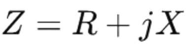
using Z=R+jX, where R is resistance and X is reactance. It would cover how phasors simplify the calculation of total impedance in series and parallel circuits.
Derivation of Sinusoidal Steady State Analysis
To lay the groundwork for sinusoidal steady-state analysis, it’s essential to derive the phasor representation and the relationships between voltage, current, impedance, and time in a clear manner. This begins with defining a sinusoid, representing it through complex exponentials, and then mapping it onto a two-dimensional complex plane.This derivation illustrates how a phasor preserves the sinusoid’s magnitude and relative phase while eliminating its time-dependent behavior. It also validates the use of concepts like impedance and Kirchhoff’s laws with phasors, as they fulfill the original circuit equations.
Such theoretical foundation is crucial for subsequent applications in steady-state analysis.
Given a sinusoidal signal as the input, the phasor representation in sinusoidal steady-state analysis is applicable to a linear time-invariant system. Sinusoidal steady-state analysis transfer function.
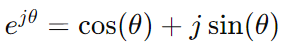
using Euler’s identities,

sinusoidal signals represented by,
𝑉𝑜𝑒𝑗(𝜔𝑡+𝜙𝑜−𝜋2)
Where,
- 𝑉𝑜 is the amplitude,
- ω is the angular frequency,
- t is time, and
- 𝜙𝑜 is the phase angle.
Expanding this expression, we get:
where
𝑉𝑠=𝑉𝑜𝑒𝑗(𝜙𝑜–𝜋2) = phasor.
Now angle Notation:-
Applications of Sinusoidal Steady-State Analysis
Sinusoidal steady-state analysis with phasors is not just a theoretical tool—it’s a practical necessity across various electrical engineering domains. Here are some key applications:
- Power Distribution Systems: In electrical grids, AC power is transmitted at a fixed frequency (e.g., 50 or 60 Hz). Phasor analysis is used to calculate voltage drops, current flows, and power losses across transformers, transmission lines, and loads. It ensures stability and efficiency by modeling impedances and phase relationships under steady-state conditions.
- Filter Design: In signal processing and communication systems, filters (e.g., low-pass, high-pass, or band-pass) are designed to manipulate sinusoidal signals. Phasors help determine the frequency response of these circuits by analyzing how impedances vary with ω, enabling precise tuning to pass or block specific frequencies.
- Resonance in RLC Circuits: Phasor analysis is critical for studying resonance, where the inductive and capacitive reactances cancel
(XL=XC), minimizing impedance and maximizing current at the resonant frequency
This phenomenon is exploited in oscillators, radio tuners, and other frequency-selective circuits.
Conclusion
Sinusoidal steady-state analysis, through the use of phasors, provides a powerful framework for simplifying the study of AC circuits. By transforming time-varying sinusoidal signals into complex numbers, engineers can efficiently analyze impedance, power, and circuit behavior under stable conditions. This method not only bridges the gap between DC and AC circuit analysis but also underpins critical applications in power systems, signal processing, and beyond. Mastering phasors and their derivations equips engineers with the tools to design and troubleshoot complex electrical systems with confidence and precision.
|
76 videos|152 docs|62 tests
|
FAQs on Sinusoidal steady state analysis: Phasors & Derivations - Network Theory (Electric Circuits) - Electrical Engineering (EE)
| 1. What is sinusoidal steady state analysis? |  |
| 2. What are phasors and how are they used in sinusoidal steady state analysis? | |
| 3. How do you derive the expressions used in sinusoidal steady state analysis? | |
| 4. What is the significance of the sinusoidal source in sinusoidal steady state analysis? | |
| 5. What are the limitations of sinusoidal steady state analysis? | |


Summary
,Objective type Questions
,Sinusoidal steady state analysis: Phasors & Derivations | Network Theory (Electric Circuits) - Electrical Engineering (EE)
,Viva Questions
,shortcuts and tricks
,video lectures
,MCQs
,Semester Notes
,Previous Year Questions with Solutions
,Sample Paper
,Exam
,Free
,study material
,Extra Questions
,past year papers
,ppt
,mock tests for examination
,Important questions
,Sinusoidal steady state analysis: Phasors & Derivations | Network Theory (Electric Circuits) - Electrical Engineering (EE)
,Sinusoidal steady state analysis: Phasors & Derivations | Network Theory (Electric Circuits) - Electrical Engineering (EE)
,practice quizzes
;


Sinusoidal steady state analysis: Phasors & Derivations Free PDF Download
Importance of Sinusoidal steady state analysis: Phasors & Derivations
Sinusoidal steady state analysis: Phasors & Derivations Notes
Sinusoidal steady state analysis: Phasors & Derivations Electrical Engineering (EE) Questions
Study Sinusoidal steady state analysis: Phasors & Derivations on the App
|
© EduRev
|
Education Revolution
|


|


