Schroedinger Equation and Expectation Values | Physics Optional Notes for UPSC PDF Download
| Table of contents |
|
| How to study QM? |
|
| The Schrodinger equation |
|
| Normalization of Ψ(x,t) |
|
| The Importance of Phases |
|
| Probability current |
|

How to study QM?
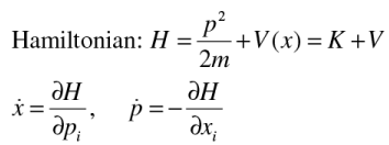
Classically the state of a particle is defined by (x,p) and the dynamics is given by Hamilton’s equations
What is a quantum mechanical state?
Coordinate and momentum is not complete in QM, needs a probabilistic predictions.
The wave function associated with the particle can represent its state and the dynamics would be given by Schrodinger equation.
However, wave function is a complex quantity!
Need to calculate the probability and the expectation values
The Schrodinger equation
Given the initial state ψ(x,0), the Schrodinger equation determines the states ψ(x,t) for all future time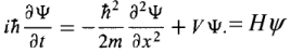 where H is the Hamiltonian of the system.
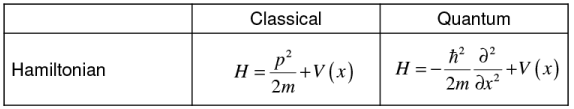
But what exactly is this "wave function", and what does it mean? After all, a particle, by its nature, is localized at a point, whereas the wave function is spread out in space (it's a function of x, for any given time t). How can such an object be said to describe the state of a particle?
Born's statistical interpretation of Ψ(x,t):
|Ψ(x,t)|² dx gives the probability of finding the particle between x and +dx, at time t or, more precisely,
|Ψ(x,t)|² dx = { probability of finding the particle between x and (x + dx), at time t. }
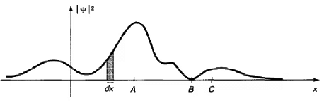 A typical wave function. The particle would be relatively likely to be found near A, and unlikely to be found near B. The shaded area represents the probability of finding the particle in the range dx.
The probability P (x,t) of finding the particle in the region lying between x and x+dx at the time t, is given by the squared amplitude P(x, t) dx = |Ψ(x,t)|²
Probability: A few definitions
Because of the statistical interpretation, probability plays a central role in quantum mechanics. The probability that x lies between a and b (a finite interval) is given by the integral of ρ(x), the probability density function: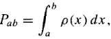
The sum of all the probabilities is 1: 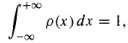
The average value of x: 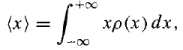
The average of a function of x: 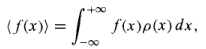
Standard deviation:
σ² ≡ ⟨(Δx)²⟩ = ⟨x²⟩ − ⟨x⟩². Δx = x − ⟨x⟩
Gaussian distribution
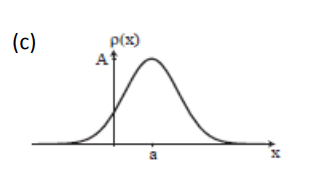
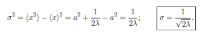
Consider the Gaussian distribution 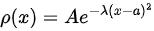 where A, a, and λ are constants. (a) Determine A, (b) Find <x>, <x2> , and σ, (c) Sketch the graph of ρ(x).
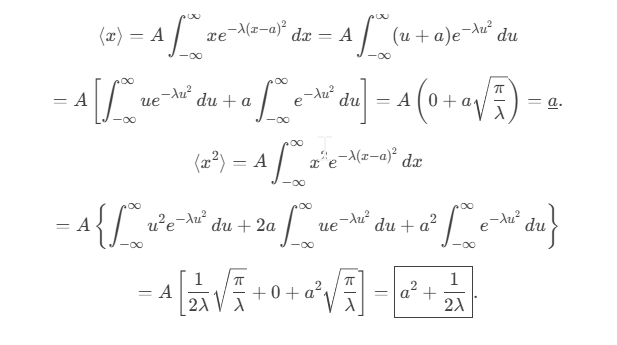
(a)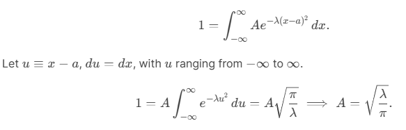 (b)
(b)
Normalization of Ψ(x,t)
|Ψ(x,t)|² is the probability density for finding the particle at point x, at time t. Because the particle must be found somewhere between x=-∞ and x=+∞ the wave function must obey the normalization condition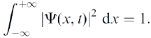 Without this, the statistical interpretation would be meaningless. Thus, there is a multiplication factor. However, the wave function is a solution of the Schrodinger eq:
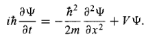
Therefore, one can't impose an arbitrary condition on ψ without checking that the two are consistent.
Interestingly, if ψ(x, t) is a solution, Aψ(x, t) is also a solution where A is any (complex) constant.
Therefore, one must pick a undetermined multiplicative factor in such a way that the Schrodinger Equation is satisfied. This process is called normalizing the wave function.
For some solutions to the Schrodinger equation, the integral is infinite; in that case no multiplicative factor is going to make it 1. The same goes for the trivial solution ψ= 0.
Such non-normalizable solutions cannot represent particles, and must be rejected.
Physically realizable states correspond to the "square-integrable" solutions to Schrodinger's equation.
What all you need is that 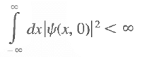
that is, the initial state wave functions must be square integrable.
Since we may need to deal with integrals of the type 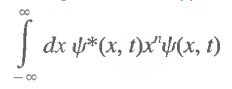
you will require that the wave functions ψ(x, 0) go to zero rapidly as x→±∞ often faster than any power of x.
We shall also require that the wave functions ψ(x, t) be continuous in x.
The Importance of Phases
The emphasis on |ψ(x, t)|² as the physically relevant quantity might lead to the impression that the phase of the wave function is of no importance. If we write ψ = Reiθ, then indeed |ψ|² = R² independent of θ. However, the linearity of the equation allows us to add solutions, as in our discussion of the electron interference pattern with two slits. We see that
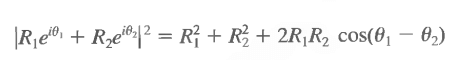
depends on the relative phase. An overall phase in the total wave function can be ignored, or chosen arbitrarily for convenience.
Example 1:A particle is represented by the wave function  ) where A, ω and a are real constants. The constant A is to be determined.
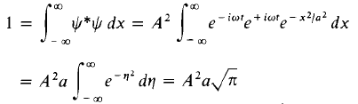
The normalized wave-function is therefore: 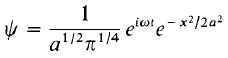
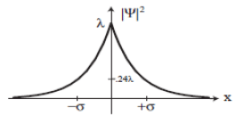
Example 2:Consider the wave function Ψ(x,t) = Ae-λ|x|e-iωt, where A, λ, and ω are positive real constants. Normalize Ψ. Sketch the graph of |Ψ|2 as a function of x.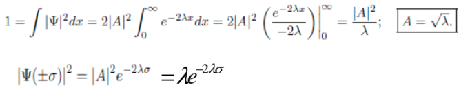
Example 3: Normalize the wave function ψ=Aei(ωt-kx), where A, k and ω are real positive constants.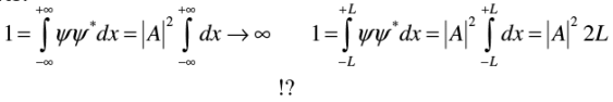
Does ψ remain normalized forever?
Suppose we have normalized the wave function at time t = 0. How do we know that it will stay normalized, as time goes on and ψ(x, t) evolves?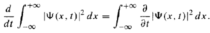 [Note that the integral is a function only of t, but the integrand is a function of x as well as t.]
By the product rule,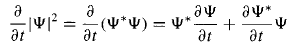 The Schrodinger equation and its complex conjugate are
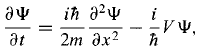 and
and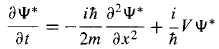 So,
So,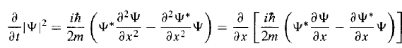 then,
then,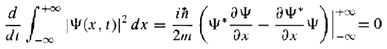 Since Ψ(x, t) must go to zero as x goes to (±) infinity - otherwise the wave function would not be normalizable. Thus, if the wave function is normalized at t = 0, it stays normalized for all future time.
The Schrodinger equation has the property that it automatically preserves the normalization of the wave function--without this crucial feature the Schrodinger equation would be incompatible with the statistical interpretation.
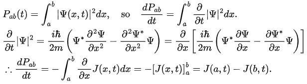
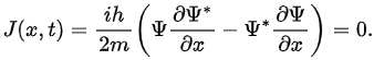
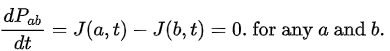
Probability current
If Pab(t) be the probability of finding the particle in the range (a < x < b), at time t, then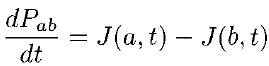 where
where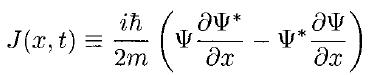
Probability is dimensionless, so J has the dimensions 1/time, and units second-1
Example: Take 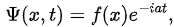 where f(x) is a real function.
So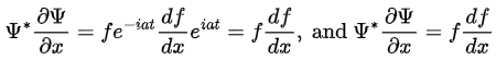
Expectation values
We are looking for expectation values of position and momentum knowing the state of the particle, i.e., the wave function ψ(x,t).
Position expectation: 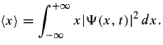 What exactly does this mean?
It does not mean that if one measures the position of one particle over and over again, the average of the results will be given by ∫ x|ψ|² dx.
On the contrary, the first measurement (whose outcome is indeterminate) will collapse the wave function to a spike at the value actually obtained, and the subsequent measurements (if they're performed quickly) will simply repeat that same result.
Rather, <x> is the average of measurements performed on particles all in the state ψ, which means that either you must find some way of returning the particle to its original state after each measurement, or else you prepare a whole ensemble of particles, each in the same state ψ, and measure the positions of all of them: <x> is the average of these results.
The position expectation may also be written as: 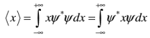
Momentum expectation:
Classically: 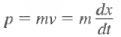 Quantum mechanically, it is <p>
Let us try: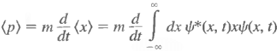
Note: d<x>/dt is the velocity of the expectation value of x, not the velocity of the particle.
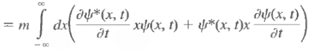
Note that there is no dx/dt under the integral sign. The only quantity that varies with time is y(x, t), and it is this variation that gives rise to a change in <x> with time. Use the Schrodinger equation and its complex conjugate to evaluate the above and we have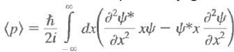 Now
Now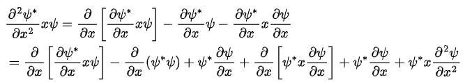 This means that the integrand has the form
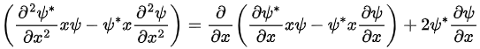
Because the wave functions vanish at infinity, the first term does not contribute, and the integral gives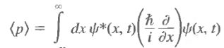
As the position expectation was represented by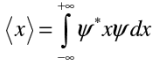
This suggests that the momentum be represented by the differential operator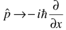
and the position operator be represented by 
To calculate expectation values, operate the given operator on the wave function, have a product with the complex conjugate of the wave function and integrate.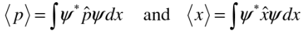
Expectation of other dynamical variables To calculate the expectation value of any dynamical quantity, first express in terms of operators x and p, then insert the resulting operator between ψ* and ψ, and integrate: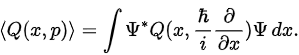
For example: Kinetic energy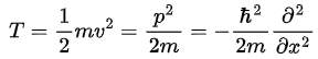
Therefore,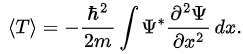
Hamiltonian: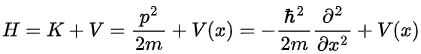
Angular momentum :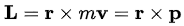
but does not occur for motion in one dimension.
Could the momentum expectation be imaginary?
The expectation value of p is always real. Let us calculate
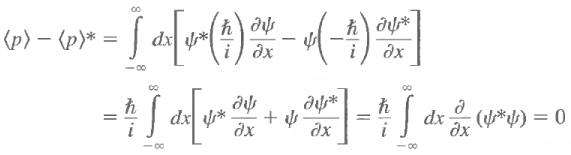
The last step follows from the square integrability of the wave functions. Sometimes one has occasion to use functions that are not square integrable but that obey periodic boundary conditions, such as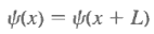 Also, under these circumstances
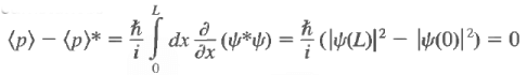
An operator whose expectation value for all admissible wave functions is real is called a Hermitian operator. Therefore, the momentum operator is Hermitian.
Product of operators
Products of operators need careful definition, because the order in which they act is important.
Example: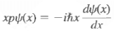 whereas
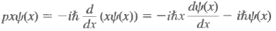
They are different. However, one can deduce 
Since this is true for all ψ(x), we conclude that we have an operator relation, which reads
This is a commutation relation, and it is interesting because it is a relation between operators, independent of what wave function this acts on. The difference between classical physics and quantum mechanics lies in that physical variables are described by operators and these do not necessarily commute.
In general one could show that: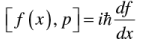
The Heisenberg Uncertainty Relations
The wave function ψ(x) cannot describe a particle that is both well-localized in space and has a sharp momentum. The uncertainty in the measurement is given by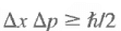 where
where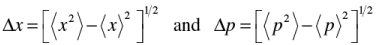
to be evaluated using position and momentum operators.
This is in great contrast to classical mechanics. What the relation states is that there is a quantitative limitation on the accuracy with which we can describe a system using our familiar, classical notions of position and momentum. Position and momentum are said to be complementary (conjugate) variables.
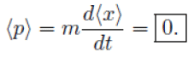
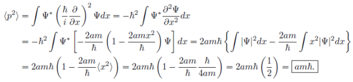
Example: A particle of mass m is in the state 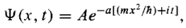 where A and a are positive real constants. (a) Find A. (b) Calculate the expectation values of <x>, <x2>, <p>, and <p2>. (d) Find σx and σp. Is their product consistent with the uncertainty principle?
(a)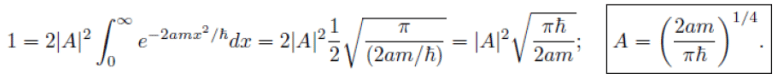 (b)
(b)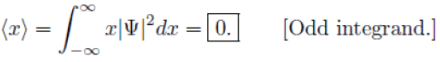
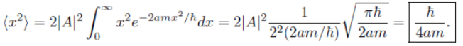
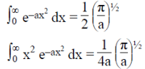
Remember:
(c)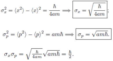 This is consistent with the uncertainty principle.
FAQs on Schroedinger Equation and Expectation Values - Physics Optional Notes for UPSC
| 1. What is the Schrödinger equation and why is it fundamental in quantum mechanics? |  |
| 2. What does normalization of the wave function Ψ(x,t) mean in quantum mechanics? | |
| 3. How does the phase of the wave function affect quantum mechanics? | |
| 4. What are expectation values in quantum mechanics and how are they calculated? | |
| 5. Why is the study of quantum mechanics important for UPSC aspirants? | |


mock tests for examination
,Schroedinger Equation and Expectation Values | Physics Optional Notes for UPSC
,Previous Year Questions with Solutions
,past year papers
,study material
,Objective type Questions
,practice quizzes
,Summary
,shortcuts and tricks
,MCQs
,Schroedinger Equation and Expectation Values | Physics Optional Notes for UPSC
,Sample Paper
,video lectures
,Semester Notes
,Schroedinger Equation and Expectation Values | Physics Optional Notes for UPSC
,Important questions
,Viva Questions
,Extra Questions
,ppt
,Free
,Exam
;


Schroedinger Equation and Expectation Values Free PDF Download
Importance of Schroedinger Equation and Expectation Values
Schroedinger Equation and Expectation Values Notes
Schroedinger Equation and Expectation Values UPSC Questions
Study Schroedinger Equation and Expectation Values on the App
|
© EduRev
|
Education Revolution
|


|


