Free Particle & Particle in a Box & Solutions of the 1D Schrodinger Equation | Physics Optional Notes for UPSC PDF Download

Gaussian Wave Packets
The Gaussian wave packet initial state is one of the few states for which both the {|x)} and {|p)} basis representations are simple analytic functions and for which the time evolution in either representation can be calculated in closed analytic form. It thus serves as an excellent example to get some intuition about the Schrodinger equation.
We define the {|x)} representation of the initial state to be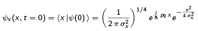
The relation between our σx and Shankar's Δx is Δx = σx√2. As we shall see, we choose to write in terms of σx because ((ΔX)2) = σx2.
Before doing the time evolution, let's better understand the initial state. First, the symmetry of (x |^(0)) in x implies (X)t=0 = 0, as follows:
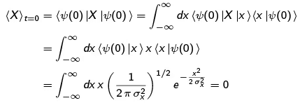
because the integrand is odd.
Second, we can calculate the initial variance ((ΔX)2)t=o: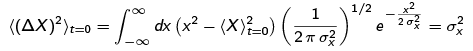
where we have skipped a few steps that are similar to what we did above for (X)t=0 and we did the final step using the Gaussian integral formulae from Shankar and the fact that (X)t=0 = 0.
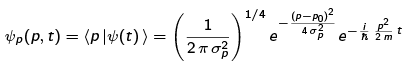
We calculate the {|p )}-basis representation of |Ψ(0)) so that calculation of (P)t=o and ((ΔP)2)t=o are easy: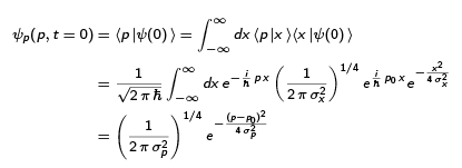
where the  comes from the normalization
  where
where  and the final step is done by completing the square in the argument of the exponential and using the usual Gaussian integral
  . With the above form for the
  -space representation of
  the calculation of (P)t=o and ((ΔP)2)t=o are calculationally equivalent to what we already did for
  yielding.
We may now calculate |Ψ(t)). Shankar does this only in the {|x)} basis, but we do it in the {|p)} basis too to illustrate how simple it is in the eigen basis of H. The result is of course
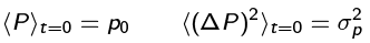
 That is, each {|p)} picks up a complex exponential factor for its time evolution. It is immediately clear that (P) and ((ΔP)2) are independent of time. Calculationally, this occurs because P, and (ΔP)2 simplify to multiplication by numbers when acting on |p) states and the time-evolution complex-exponential factor cancels out because the two expectation values involve (Ψ | and Ψ). Physically, this occurs because the P operator commutes with H; later, we shall derive a general result about conservation of expectation values of operators that commute with the Hamiltonian. Either way one looks at it, one has
Let's also calculate the {|x)} representation of |Ψ(t)). Here, we can just use our propagator formula, which tells us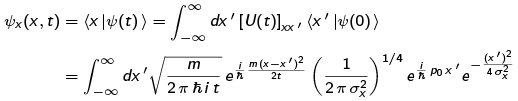
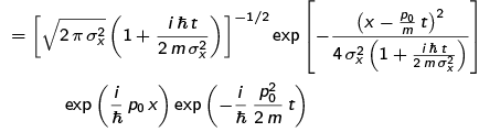
where we do the integral in the usual fashion, by completing the square and using the Gaussian definite integral.
The probability density in the {|x)} basis is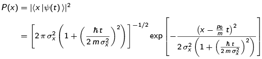 Because the probability density is symmetric about
  , it is easy to see that
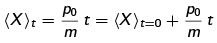 i.e., the particle’s effective position moves with speed po/m, which is what one expects for a free particle with initial momentum po and mass m.
The variance of the position is given by the denominator of the argument of the Gaussian exponential (one could verify this by calculation of the necessary integral),
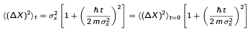
The position uncertainty grows with time because of the initial momentum uncertainty of the particle - one can think of the {|p)} modes with p > po as propagating faster than po/m and those with p < po propagating more slowly, so the initial wavefunction spreads out over time. In the limit of large time 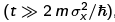 , the uncertainty
  grows linearly with time. The "large time" condition can be rewritten in a more intuitive form:
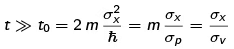
where σv = σp/m is the velocity uncertainty derived from the momentum uncertainty. So, t0 is just the time needed for the state with typical velocity to move the width of the initial state. We should have expected this kind of condition because σx and  are the only physical quantities in the problem. Such simple formulae can frequently be used in quantum mechanics to get quick estimates of such physical phenomena; we shall make such use in the particle in a box problem.
Position-Momentum Uncertainty Relation
Before leaving the free particle, we note an interesting relationship that appeared along the way. Recall that, because the position and momentum operators do not commute, 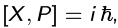 , no state is an eigenstate of both. If there is no uncertainty in one quantity because the system is in an eigenstate of it, then the uncertainty in the other quantity is in fact infinite. For example, a perfect position eigenstate has a delta-function position-space representation, but it then, by the alternative representation of the delta function, we see that it is a linear combination of all position eigenstates with equal weight. The momentum uncertainty will be infinite. Conversely, if a state is a position eigenstate, then its position-space representation has equal modulus everywhere and thus the position uncertainty will be infinite.
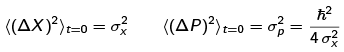
When we considered the Gaussian wave packet, which is neither an eigenstate of X nor of P, we found that the t = 0 position and momentum uncertainties were
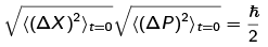
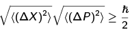
 Hence, at t = 0, we have the uncertainty relation
 We saw that, for t > 0, the position uncertainty grows while the momentum uncertainty is unchanged, so in general we have
 We will later make a general proof of this uncertainty relationship between noncommuting observables.
The Hamiltonian
A "box” consists of a region of vanishing potential energy surrounded by a region of infinite potential energy:
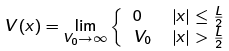 It is necessarily to include the limiting procedure so that we can make mathematical sense of the infinite value of the potential when we write the Hamiltonian. Classically, such a potential completely confines a particle to the region |x| < L/2. We shall find a similar result in quantum mechanics, though we need a bit more care in proving it.
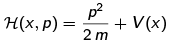
The classical Hamiltonian is
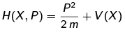
 Postulate 2 tells us that the quantum Hamiltonian operator is
 Next, we want to obtain an eigenvalue-eigenvector equation for H. For the free particle, when V(X) was not present, it was obvious we should work in the {|p)} basis because H was diagonal there, and then it was obvious how P acted in that basis and we could write down the eigenvalues and eigenvectors of H trivially. We cannot do that here because V(X) and hence H is not diagonal in the {|p)} basis. Moreover, regardless of basis, we are faced with the problem of how to interpret V(X). Our usual power-series interpretation fails because the expansion is simply not defined for such a function — its value and derivatives all become infinite for |x| > L/2.
Shankar glosses over this issue and jumps to the final differential equation; thereby ignoring the confusing part of the problem! We belabor it to make sure it is clear how to get to the differential equation from H and the postulates. The only sensible way we have to deal with the above is to write down matrix elements of H in the {|x)} basis because our Postulate 2 tells us explicitly what the matrix elements of X are in this basis. Doing that, we have
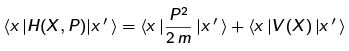 Let's look at each term separately. For the first term, since it is quadratic in P, let's insert completeness to get the P's separated:

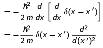 where in last step we used Equation
 For the second term, we can approach it using a limiting procedure. Suppose V (X ) were not so pathological; suppose it has a convergent power series expansion
 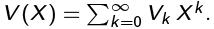 Then, we would have
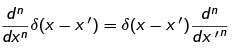
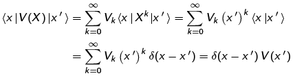 where we have allowed X to act to the right on |x'). This is not a strict application of Postulate 2; if one wants to be really rigorous about it, one ought to insert completeness relations like we did for P2. For example, for X2 we would have
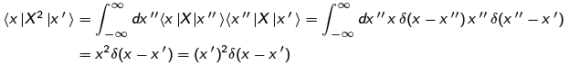 For Xk, we have to insert k -1 completeness relations and do k- 1 integrals. The result will be of the same form.
The key point in the above is that we have figured out how to convert the operator function V(X) into a simple numerical function V(x) when V(X) can be expanded as a power series. To apply this to our non-analytic V(X), we could come up with an analytic approximation that converges to the non-analytic one as we take some limit. (One could use a sum of tan-1 or tanh functions, for example.) The point is that if we used the expansion and then took the limit, we would obtain a result identical to the above. So we write
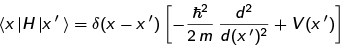
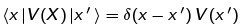 With the above results, we have that the matrix elements of H are given by:
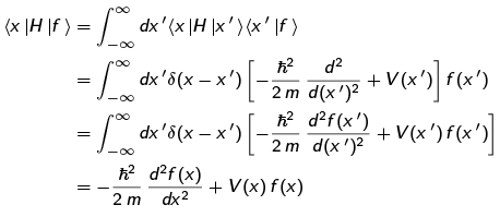
 Thus, for an arbitrary state | f), we have that (using completeness as usual)
Particle in a finite square well
A slightly more realistic model of a confined particle is given by the finite square well potential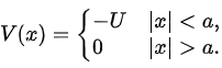
- a crude model of the Coulomb potential of a charged nucleus. We will look for bound state solutions - normalisable solutions - as opposed to unnormalisable scattering solutions, whose physical interpretation we will discuss later.
A solution of energy E obeys
If E > 0, the solution for |x| > a takes the form 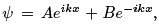 where
where . This is unnormalisable.
So we require E < 0. We will assume that E > —U, i.e. that |E| < U, since we do not expect there to be solutions with energy lower than the minimum potential.
Exercise: Verify that indeed there are no such solutions.
Let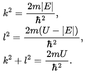 For |x| > a we have
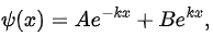 and normalisability implies that
 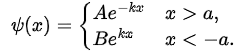 For |x| < a we have
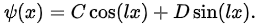
Since we know that the states of definite parity span the space of all bound states, we can solve separately for even and odd parity states to get a complete spanning set of solutions.
Consider the even parity solutions. If Ψ(x) = Ψ(—x) we have:
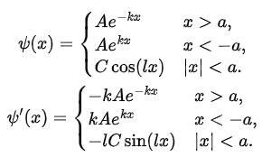
As Ψ and are continuous at x = ±a, we find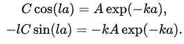
This gives
k = ltan(la)
or
(ka) = (la) tan (la)
and from (4.34) we have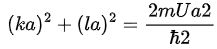 We can solve these last two equations graphically.
The odd parity bound states (if any exist) can be similarly obtained.The finite square well illustrates a general feature of quantum potentials V(x) such that V(x) → 0 as x→ ±∞. The time-independent SE has two linearly independent solutions.
For E > 0, these take the form of scattering solutions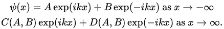
For E < 0, they have the form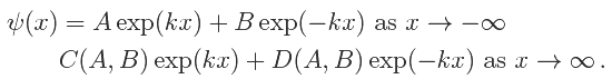
Here C(A, B) and D(A, B) are linear in A and B, and depend also on k and on the parameters defining V(x).
Only for special values of E < 0 can we find solutions such that B = 0 and C(A, B) = 0, as required for normalisability. For the remaining values of E < 0, the solutions blow up exponentially as x → -∞ or as x → ∞ (or both) and are unphysical: neither bound states nor scattering solutions. [These asymptotically exponential functions are not physically meaningful: they are not normalisable and do not define eigenfunctions of H.]
The quantum harmonic oscillator
has potential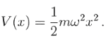 This is a particularly important example for several reasons.
First, it is not only solvable but (as we will see later) has a very elegant solution that explains some important features of quantum theory.
Second, generic symmetric potentials in 1D are at least approximately. To see this, consider a potential V(x) taking a minimum value Vmin at xmin and symmetric about xmin. Writing y = x — xmin, we have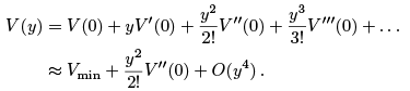 Renormalising the potential so that Vmin = 0, and taking V"(0) = mω2. (If V"(0) = 0 this argument does not hold, but even in this case the harmonic oscillator potential can be a good qualitative fit. See for example comments below on approximating a finite square well potential by a harmonic oscillator potential.)
In fact, we can show something more general. Suppose we have a system with n degrees of freedom that has a unique stable equilibrium. Then the small oscillations about equilibrium can be approximated by n independent harmonic oscillators. This means that solving the harmonic oscillator allows us to give a quantum description of molecules excited by radiation (and hence understand the greenhouse effect and many other phenomena) and of the behaviour of crystals and other solids.
Third, the harmonic oscillator plays an even more fundamental role in quantum field theory, where we understand particles as essentially harmonic oscillator excitations of fields. Our entire understanding of matter and radiation is thus based on the quantum harmonic oscillator!
To obtain the stationary states of the quantum harmonic oscillator we need to solve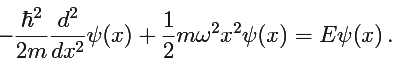 We define
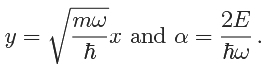 We have
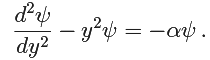 If ψ ∼ exp(−1/2 y2), then ψ' ∼ −y exp(−1/2 y2) and ψ'' ∼ y2 exp(−1/2 y2) to leading order, which means that ψ'' − y2ψ ∼ (y2 − y2) exp(−1/2 y2) satisfies to leading order. Similarly ψ ∼ yn exp(−1/2 y2) satisfies (4.47) to leading order. This suggests considering power series solutions of the form.
We define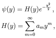 and trying to match the coefficients am to produce an exact solution.
we get
Ψ"+ (a - y2)Ψ = 0
and substituting, we get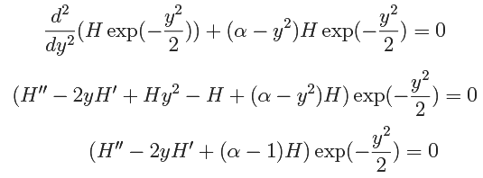 We have
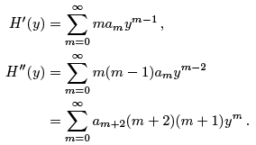
So, we get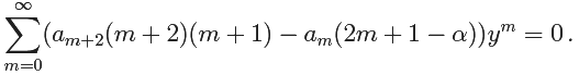 This must be true for ally, so each coefficient of ym must vanish:
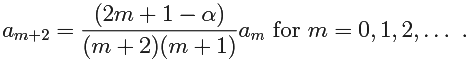 which determines the am for m ≥ 2 in terms of a0 and a1.
For large m, gives 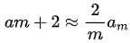 , which asymptotically describes the coefficients of
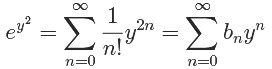
where for n odd we have bn = 0and for n even we have
So, if the power series is infinite, we expect
for some nonzero constant C: i.e. that  as y → ∞. This implies that
which is not normalisable. We can justify this rigorously by noting that, for any ε > 0, there exists some integer m0 such that for all m ≥ m0 we have
Hence we have that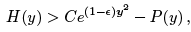
where C = am0 ≠ 0 and P(y) is a polynomial of degree ≤ m0. This implies that there exists a y0 such that for all y ≥ y0
we have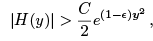 and hence
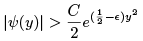 So indeed ψ(y) diverges as y → ∞, and in particular ψ is not normalisable.
We thus need the power series to be truncated to a polynomial in order to find normalisable physical solutions. Again, we can consider fixed (even and odd) parity solutions separately:
- Even parity: a0 ≠ 0, a1 = 0, α = 2m + 1 for some even m.
- Odd parity: a0 = 0, a1 ≠ 0,α = 2m + 1 for some odd m.
So the physical solutions are given by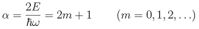 i.e
i.e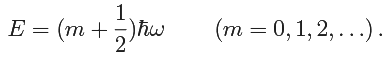
The harmonic oscillator has energy levels equally spaced, separated by  with minimum (orzero-point) energy
  The polynomials Hn(y) corresponding to the physical solutions with energy
  are the Hermite polynomials of degree n. We can obtain them explicitly 17 from (4.65), using conventional normalisations:
 The corresponding wavefunctions are thus (up to normalisation)
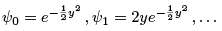
FAQs on Free Particle & Particle in a Box & Solutions of the 1D Schrodinger Equation - Physics Optional Notes for UPSC
| 1. What is a Gaussian wave packet and how does it relate to quantum mechanics? |  |
| 2. How does the position-momentum uncertainty relation work in quantum mechanics? | |
| 3. What is the Hamiltonian for a free particle, and how is it derived? | |
| 4. What are the boundary conditions for a particle in a box in quantum mechanics? | |
| 5. How do you solve the 1D Schrödinger equation for a particle in a box? | |


ppt
,Extra Questions
,Free Particle & Particle in a Box & Solutions of the 1D Schrodinger Equation | Physics Optional Notes for UPSC
,mock tests for examination
,Important questions
,video lectures
,Viva Questions
,Free
,Previous Year Questions with Solutions
,Semester Notes
,study material
,Sample Paper
,Summary
,Objective type Questions
,MCQs
,Exam
,Free Particle & Particle in a Box & Solutions of the 1D Schrodinger Equation | Physics Optional Notes for UPSC
,Free Particle & Particle in a Box & Solutions of the 1D Schrodinger Equation | Physics Optional Notes for UPSC
,shortcuts and tricks
,practice quizzes
,past year papers
;


Free Particle & Particle in a Box & Solutions of the 1D Schrodinger Equation Free PDF Download
Importance of Free Particle & Particle in a Box & Solutions of the 1D Schrodinger Equation
Free Particle & Particle in a Box & Solutions of the 1D Schrodinger Equation Notes
Free Particle & Particle in a Box & Solutions of the 1D Schrodinger Equation UPSC Questions
Study Free Particle & Particle in a Box & Solutions of the 1D Schrodinger Equation on the App
|
© EduRev
|
Education Revolution
|


|


